Unit 2.3 - Theory of Price and Output Determination
Equilibrium Condition of Firm & Industry Under PCM
The main objective of a firm under PCM is to maximize the profit. The profit maximization condition of the firm is also called equilibrium condition of a firm.
Graphical Method
1. Traditional Approach: Total Revenue – Total Cost (TR-TC) Approach
In this approach, TR and TC are under consideration. Since, the objective of the firm is profit maximization. profit is the difference between TR and TC. We have, B = TR – TC
a. Abnormal (excess) profit: TR>TC ⇒ B>0
b. Normal profit (cost recovering revenue): Normal profit is included in the cost TR=TC ⇒B=0
c. Loss: TR<TC ⇒ B<0
The profit is maximized at the output
where there is the biggest gap or highest difference between TR & TC, which
is given by PM in the figure. TR-TC approach is shown in figure below:

In
figure, TR curve under PCM is a straight line, positively sloped and passes
through origin. It is because of the price being constant. TC curve is inverse
S-shaped comprising TVC and TFC. TR curve intersects TC curve at points A and
B. At point A output is Q1
and at point B output is Q3. In the figure, before the output level
Q1 and after output Q3, there is loss because TR curve
lies below the TC curve (i.e. TR<TC). The output between Q1 and Q3,
there is TR>TC which shows there is profit. The biggest gap between TR and
TC i.e. MP is at output level Q2 where profit is maximum. Thus, the
output at this position gives the equilibrium output of the firm.
Profit curve (i.e. B-curve)
is drawn measuring the gap between TR and TC curves. Before the output Q1
and after the output Q3 the B-curve
lies below X-axis. It shows there is loss to the firm. Between outputs from Q1
to Q2 the B-curve
rises, showing that there is profit which increases as increase in output. In
the similar fashion, the B-curve
starts to fall from the outputs between Q2 and Q3. The
maximum profit (Q2N) is at the output Q2. The profit
curve reaches at maximum point N when output is 0Q2.
|
Q |
TR |
TC |
B |
|
5 |
15 |
18 |
-3 |
|
6 |
20 |
22 |
-2 |
|
7 |
25 |
26 |
-1 |
|
8 |
30 |
27 |
3 |
|
9 |
35 |
30 |
5 Max |
|
10 |
40 |
38 |
2 |
Example : In this
example producer is in equilibrium at 9th unit.
2. Modern Approach: Marginal Revenue-Marginal Cost (MR-MC) Approach
In this approach MR and MC are used to determine the profit maximization conditions. The profit maximization conditions are mentioned below in MR-MC approaches:
a. Necessary Condition : MR = MC
b. Sufficient Condition: MC cuts MR from below (Slope of MC>Slope of MR)

In figure, both the conditions are
fulfilled at point E not the point A.
Between the point A & E, MC is lower
than MR. Therefore it is profitable for the firm to expand output up to 0Q
level of output.
At 0Q level of output, the firm will be in
equilibrium because above mentioned two conditions are fulfilled. This is the
point of maximum profit of the firm. Thus, the firm will go on expanding up to
0Q but it is not profitable to produce more than 0Q level of output because
beyond 0Q level of output MC is greater than MR.
Summary
a. If
MC<MR → expanding output is profitable
b. If MC =
MR→ short run profit is maximum
c. If
MC<MR → reducing output is may prevent loss
|
Q |
P |
TR |
TC |
MR |
MC |
B |
|
1 |
10 |
10 |
11 |
10 |
11 |
-1 |
|
2 |
10 |
20 |
21 |
10 |
10 |
-1 |
|
3 |
10 |
30 |
30 |
10 |
9 |
0 |
|
4 |
10 |
40 |
38 |
10 |
8 |
2 |
|
5 |
10 |
50 |
48 |
10 |
10 |
2 |
|
6 |
10 |
60 |
59 |
10 |
11 |
1 |
Equilibrium
Condition Under Monopoly
The main objective of a firm under monopoly also is to maximize the profit. The profit maximization condition of the firm is also called equilibrium condition of a firm.
Graphical Method
1. Traditional Approach: Total Revenue – Total Cost (TR-TC) Approach
In this approach, TR and TC are under consideration. Since, the objective of the firm is profit maximization. Profit is the difference between TR and TC. We have, B = TR – TC
a. Abnormal (excess) profit: TR>TC ⇒B>0
b. Normal profit (cost recovering revenue): Normal profit is included in the cost TR=TC ⇒B=0
c. Loss: TR<TC ⇒B<0
The profit is maximized at the output
where there is the biggest gap or highest difference between TR & TC, which
is given by PM in the figure. TR-TC approach is shown in figure below:

In
figure, TR curve under monopoly is bell shaped and passes through origin. It
shows the TR initially rises, reaches at maximum and then after falls when
quantity sold increases. It is because of the inverse relationship between
price and quantity. TC curve is inverse S-shaped comprising TVC and TFC. TR
curve intersects TC curve at points A and B.
At point A output is Q1 and at point B output is Q3.
In the figure, before the output level Q1 and after output Q3,
there is loss because TR curve lies below the TC curve (i.e. TR<TC). The
output between Q1 and Q3, there is TR>TC which shows
there is profit. The biggest gap between TR and TC i.e. MP is at output level Q2
where profit is maximum. Thus, the output at this position gives the
equilibrium output of the firm.
Profit curve (i.e. B-curve) is drawn measuring the gap between TR and TC curves. Before the output Q1 and after the output Q3 the B-curve lies below X-axis. It shows there is loss to the firm. Between outputs from Q1 to Q2 the B-curve rises, showing that there is profit which increases as increase in output. In the similar fashion, the B-curve starts to fall from the outputs between Q2 and Q3. The maximum profit (Q2N) is at the output Q2. The profit curve reaches at maximum point N when output is 0Q2.
2. Modern Approach: Marginal Revenue-Marginal Cost (MR-MC) Approach
In this approach MR and MC are used to determine the profit maximization conditions. The profit maximization conditions are mentioned below in MR-MC approaches:
a. Necessary Condition : MR = MC
b. Sufficient Condition: MC cuts MR from below (Slope of MC>Slope of MR)

In figure, both the conditions are
fulfilled at point E not the point A.
Between the point A & B, MC is lower
than MR. Therefore it is profitable for the firm to expand output up to 0Q
level of output.
At 0Q level of output, the firm will be in
equilibrium because above mentioned two conditions are fulfilled. This is the
point of maximum profit of the firm. Thus, the firm will go on expanding up to
0Q but it is not profitable to produce more than 0Q level of output because
beyond 0Q level of output MC is greater than MR.
Summary
a. If
MC<MR → expanding output is profitable
b. If MC =
MR→ short run profit is maximum
c. If MC<MR → reducing output is may prevent loss
Pricing
Under PCM-Equilibrium of Firm in SR & LR (MR-MC Approach)
Short-Run Equilibrium of Firm under PCM
Short run is a period of time in which the
firm can change its level of output by changing variable factors of production
i.e. it is a period in which market supply cannot be varied according to change
in market demand due to lack of sufficient time.
A firm is said to be in equilibrium when it maximizes its profit. The output which gives maximum profit to the firm is called equilibrium output. All the firms in the industry are price takers. The following conditions must be fulfilled for a firm to be in equilibrium.
i. MC = MR
ii. MC cut MR from below i.e. slope of MC curve>slope of MR curve
The firm is in short-run equilibrium does not necessarily mean that it makes abnormal profits. Whether the firm makes abnormal profit or normal profit or losses depends on the level of AC and AR i.e. price and AC. There are three types of firms which are in equilibrium in the short-run. They are given below.
1. Equilibrium of a Firm with Abnormal Profit (P>AC)
If price is greater than AC of the firm at
the point of equilibrium, the firm is enjoying abnormal profit. It is shown in
the following diagram.

In Figure, P = 0P, AC = QB (=0C) and Q =
0Q
We know that, B = TR – TC = (P×Q) – (AC×Q) = (0P×0Q) – (0C×0Q) = 0PEQ – 0CBQ = PCBE
2. Equilibrium of a Firm with Normal Profit (P=AC)
If the
price is equal to AC (P=AC), at the point of equilibrium the firm is in
equilibrium with normal profit. The normal profit is included in AC. The
equilibrium of the firm with normal profit is explained with the help of
following diagram.

The firm is in equilibrium at point E,
where MR = MC and MC cuts MR from below. The equilibrium price and output are
0P and 0Q respectively. From the equilibrium point, the possible minimum point
of AC curve just equal to AR curve i.e. AR = AC. It indicates that firm B
enjoys only normal profit.
From Figure, P = 0P, AC = 0P and Q = 0Q
We know that, B = TR – TC = (P×Q) – (AC×Q) = (0P×0Q) – (0P×0Q) = 0PEQ – 0PEQ = 0
3. Equilibrium of a Firm with Loss (P<AC)
If the
price is less than AC (P<AC) at the point of equilibrium, the firm is facing
a loss. The following figure shows the equilibrium of the firm in short-run.

From Figure, P = 0P, AC = 0C and Q = 0Q
We know that, B = TR –
TC = (P×Q) – (AC×Q) = (0P×0Q) – (0C×0Q) = 0PEQ – 0CBQ = – PEBC
Short-Run
Equilibrium of Industry under PCM
Industry is the group of firms producing
homogenous products. Industry is in equilibrium at that price where quantity
demand is equal to quantity supply. So, the job of an industry is to determine
the price of the product.
In an industry there are large numbers of
firms producing homogenous product. All the firms under the industry are in
equilibrium. Due to cost conditions of the firm all the firms are not enjoying
abnormal profit. There are three types of firms in the industry. Some firms are
in equilibrium with abnormal profit, some firms are in equilibrium with normal
profit and some firms may be in equilibrium with loss also. The sum of total
outputs of all these three types of firms is equal to the output of the
industry. The firm A represents those types of firms which are in equilibrium
with abnormal profit, firm B represents those types of firms which are in
equilibrium with profit, and firm C represents those types of firms which are
in equilibrium with loss.
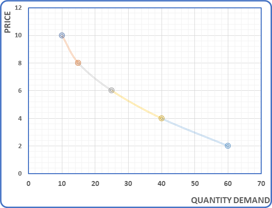
Price and output of an industry is determined
by intersection of negatively sloped demand curve and positively sloped supply
curve of the industry. It is shown in the figure. All the firms in the industry
are price takers not price makes because each firms possess perfectly elastic
demand curve. It can be explained with the help of following graph.

In the
figure, where D=S industry is in equilibrium at point E and equilibrium price
is P and quantity is Q. This price remains constant for all the firms. If the
price rises to higher level excess supply situation (i.e. S>D) is created.
When market faces excess supply situation the price must decrease to clear it
and again reaches at the original position P. When the price is below the
equilibrium, it creates the excess demand situation (i.e. D>S). It causes
increase in price again to the original position P. Thus, it remains constant
at P if demand and supply curves are the same. The equilibrium output of the
industry also remains same at point Q. It is the horizontal summation of
quantity by all the firms in the industry.
All the firms are price takers not price
makers and a single firm cannot affect the market price of the product. At this
price firm determines their output.
The output produced by firm A is 0QA,
firm B is 0QB and firm C is 0QC.
The total output, 0Q = 0QA +0QB +0QC
Long-Run Equilibrium of Firm under PCM
Long-run is a period of time in which the
firm can change its level of output by changing all the factors of production
i.e. it is a period in which market supply can be adjusted according to change
in market demand due to the availability of sufficient time. If there is
abnormal profit in the short run, more firms are attracted into the market and
output increases consequently price fall to normal level in the long-run.
Similarly, if there is loss in short-run. The firms either improve or change
their plants to reduce cost or exit from the industry so that the remaining
firms enjoy normal profit only. In this way all the firms are in equilibrium
with normal profit in the long-run.
All the
firms in the industry are price takers. All the firms in the industry get
normal profit in the long-run. All the firms are able to utilize their plants
at optimal capacity i.e. the minimum point of LAC curve just equal LAR or P.
The following condition must be fulfilled for a firm to be in equilibrium.
i. LMR = LMC i.e long-run MR must be equal to
long-run MC curve
ii. LMC curve cuts LMR from below
The long-run equilibrium of firm under PCM
can be explained with the help of following graph.

The firm is in equilibrium at point E in the long-run, where LMR= LAR =LMC=LAC= SMC=SAC and LMC curve cuts LMR curve from below. The equilibrium price and output are 0P and 0Q respectively. The minimum point of LAC is just equal to AR line i.e. LAC = LAR, which indicates that the firm is able to earn only normal profit in the long-run.
Long-Run Equilibrium of the Industry under PCM
Long-run
is a period of time in which the firm can change its level of output by
changing all the factors of production i.e. it is a period in which market
supply can be adjusted according to change in market demand due to the
availability of sufficient time. Industry is the group of firms which is
equilibrium at that price where quantity demand is equal to the quantity
supply. It can be explained with the help of following graph.

In the figure, The firms will be
equilibrium at point e in the long-run, where LMC=LMR and LMC curve cuts LMR
from below. The firm is able to earn only normal profit in the long-run. The
total output of the industry is the sum of the outputs of the firms. Similarly,
Industry will be in equilibrium at point E, where demand curve (D) is equal to
supply curve (S). The equilibrium price and output are 0P and 0Q respectively.
Pricing Under Monopoly-Equilibrium of Firm in SR & LR (MR-MC Approach)
Short-Run Equilibrium of Monopoly
Short run is a period of time in which the
monopoly firm can change its level of output by changing variable factors of
production. No doubt, fixed factors will also be utilized to their maximum
capacity to increase the output. Similarly, when demand decreases, the
monopolist will reduce his output by reducing variable factors and by slowing
down the intensive use of fixed factors.
A monopoly firm is said to be in equilibrium when it maximizes its profit. The output which gives maximum profit to the monopoly firm is called equilibrium output. The following conditions must be fulfilled for a monopoly firm to be in equilibrium.
i. MC = MR
ii. MC cut MR from below i.e. slope of MC curve>slope of MR curve
The monopoly firm is in short-run equilibrium does not necessarily mean that it makes abnormal profits. Whether the monopoly firm makes abnormal profit or normal profit or losses depends on the level of AC and AR i.e. price and AC. There are three types of monopoly firms which are in equilibrium in the short-run. They are given below.
1. Equilibrium of a Monopoly Firm with Abnormal Profit (P>AC)
If price is greater than AC of the firm at
the point of equilibrium, the firm is enjoying abnormal profit. It is shown in
the following diagram.
")
The firm is in equilibrium at point E
where MC = MR and MC cuts MR from below. The equilibrium price and output are
0P and 0Q respectively. Form the equilibrium point, the possible minimum point
of AC curve lies below the AR curve i.e. AR>AC. It indicates that the firm
enjoys abnormal profit equal to shaded area PABC.
In Figure, P = 0P, AC = QB (=0C) and Q =
0Q
We know that, B = TR – TC = (P×Q) – (AC×Q) = (0P×0Q) – (0C×0Q) = 0PAQ – 0CBQ = PABC
2. Equilibrium of Monopoly with Normal Profit (P=AC)
If the price or average revenue is equal
to AC (P=AC), at the point of equilibrium the firm is in equilibrium with
normal profit. The normal profit is included in AC. The equilibrium of the firm
with normal profit is explained with the help of following diagram.
")
The firm is in equilibrium at point E,
where MR = MC and MC cuts MR from below. The equilibrium price and output are
0P and 0Q respectively. From the equilibrium point, the possible minimum point
of AC curve just equal to AR curve i.e. AR = AC. It indicates that monopoly
firm is just relaxed on normal profit.
From Figure, P = 0P, AC = 0P and Q = 0Q
We know that, B = TR – TC = (P×Q) – (AC×Q) = (0P×0Q) – (0P×0Q) = 0PAQ – 0PAQ = 0
3. Equilibrium of Monopoly with Loss (P<AC)
If the
price is less than AC (P<AC) at the point of equilibrium, the firm is facing
a loss. The following figure shows the equilibrium of the firm in short-run.
")
The firm is in equilibrium at point E
where MR = MC and MC cuts MR from below. The equilibrium price and output are
0P and 0Q respectively. From the equilibrium point, the possible minimum point
of AC curve lies above the AR curve i.e. AR<AC. It indicates that monopoly
firm is bearing losses equal to shaded area PABC.
From Figure, P = 0P, AC = 0C and Q = 0Q
We know that, B = TR – TC = (P×Q) – (AC×Q) = (0P×0Q) – (0C×0Q) = 0PAQ – 0CBQ = – PABC
Long-Run Equilibrium of Monopoly
Long-run is a period of time in which the
firm can change its level of output by changing all the factors of production
i.e. it is a period in which market supply can be adjusted according to change
in market demand due to the availability of sufficient time.
In the long-run, a monopolist earns super-normal profit by adjusting both price as well as output and utilizing the plant size at optimal capacity. Equilibrium condition with super-normal profit refers to a situation where LAR>LAC. However, the monopolist can operate his plant at any level which depends on market demand (AR curve).
The following condition must be fulfilled for a firm to be in equilibrium.
i. LMR = LMC i.e long-run MR must be equal to long-run MC curve
ii. LMC curve cuts LMR from below
The long-run equilibrium of firm under
monopoly can be explained with the help of following graph.

The firm is in equilibrium at point E in
the long-run, where LMR=LAR=LMC=LAC=SMC=SAC and LMC curve cuts LMR curve from
below. The equilibrium price and output are 0P and 0Q respectively. From the
equilibrium point, the possible minimum point of LAC lies below the AR line
i.e. LAC < LAR, which indicates that the monopolist is able to enjoy
super-normal profit equal to shaded area PABC in the long-run.
In Figure, P = 0P, LAC = QB (=0C) and Q =
0Q
We know that, B = TR – TC = (P×Q) – (LAC×Q) = (0P×0Q) – (0C×0Q) = 0PAQ – 0CBQ = PABC

Comments
Post a Comment
If you have any doubt, Please let me know !